Ribbon Function in Excel 2016
Ribbon
Excel selects the ribbon's Home tab when you open it. Learn how to use the ribbon.
Tabs
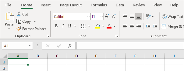
The tabs on the ribbon are: File, Home, Insert, Page layout, Formulas, Data, Review, View and Help. The Home tab contains the most frequently used commands in Excel.
 |
| KarimExcelVBA |
Groups
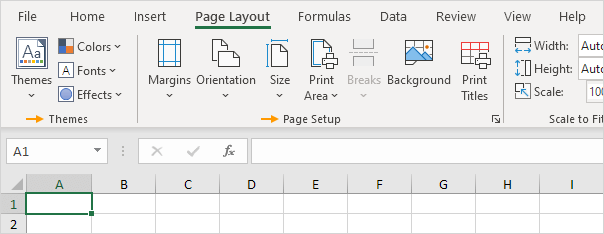
Each tab contains groups of related commands. For example, the Page Layout tab contains the Themes group, the Page Setup group, etc.
Use the Ribbon
Let's use the ribbon to insert a table. Tables allow you to analyze your data in Excel quickly and easily.
1. Click any single cell inside a data set.
2. On the Insert tab, in the Tables group, click Table.
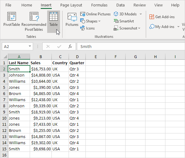
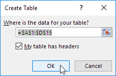
3. Excel automatically selects the data for you. Check 'My table has headers' and click on OK.
Result. Excel creates a nicely formatted table for you.
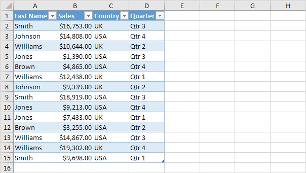
Note: use the drop-down arrows to quickly sort and filter. Visit our chapter about tables to learn more about this topic.
Collapse the Ribbon
You can collapse the ribbon to get extra space on the screen. Right click anywhere on the ribbon, and then click Collapse the Ribbon (or press CTRL + F1).
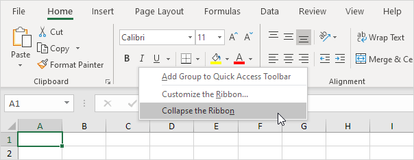
Result.

Quick Access Toolbar
1:- Quick Access Toolbar 101
2:- Commands Not in the Ribbon
If you use an Excel command frequently, you can add it to the Quick Access Toolbar. By default, the Quick Access Toolbar contains four commands: AutoSave, Save, Undo and Redo.
1:- Quick Access Toolbar 101
2:- Commands Not in the Ribbon
If you use an Excel command frequently, you can add it to the Quick Access Toolbar. By default, the Quick Access Toolbar contains four commands: AutoSave, Save, Undo and Redo.
Quick Access Toolbar 101
To add a command to the Quick Access Toolbar, execute the following steps.
1. Right click the command, and then click Add to Quick Access Toolbar.
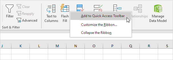
2. You can now find this command on the Quick Access Toolbar.
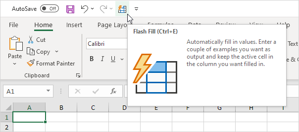
3. To remove a command from the Quick Access Toolbar, right click the command, and then click Remove from Quick Access Toolbar.
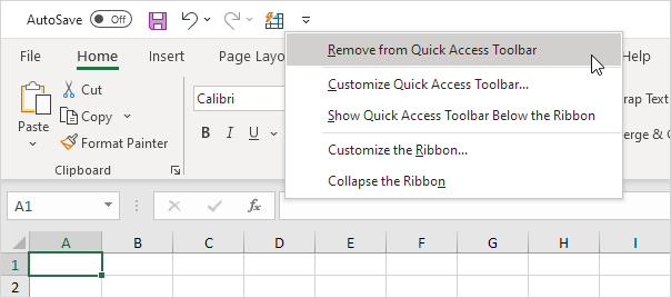
To add a command to the Quick Access Toolbar, execute the following steps.
1. Right click the command, and then click Add to Quick Access Toolbar.

2. You can now find this command on the Quick Access Toolbar.

3. To remove a command from the Quick Access Toolbar, right click the command, and then click Remove from Quick Access Toolbar.

Commands Not in the Ribbon
To add a command to the Quick Access Toolbar that isn't on the ribbon, execute the following steps.
1. Click the down arrow.
2. Click More Commands.
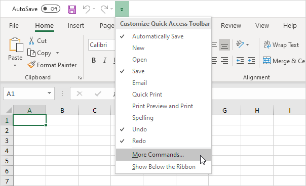
3. Under Choose commands from, select Commands Not in the Ribbon.
4. Select a command and click Add.
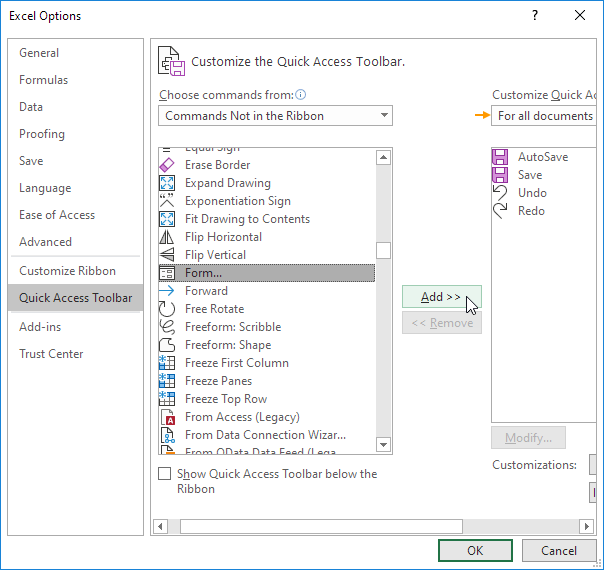
Note: by default, Excel customizes the Quick Access Toolbar for all documents (see orange arrow). Select the current saved workbook to only customize the Quick Access Toolbar for this workbook.
5. Click OK.
6. You can now find this command on the Quick Access Toolbar.
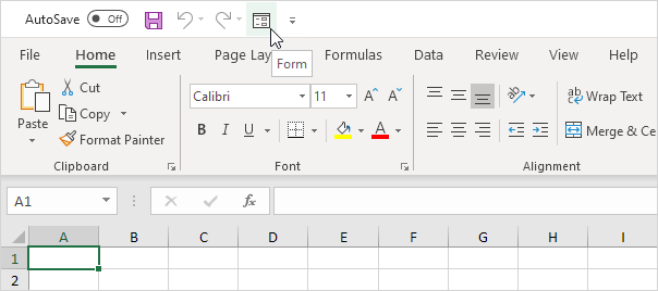
To add a command to the Quick Access Toolbar that isn't on the ribbon, execute the following steps.
1. Click the down arrow.
2. Click More Commands.

3. Under Choose commands from, select Commands Not in the Ribbon.
4. Select a command and click Add.

Note: by default, Excel customizes the Quick Access Toolbar for all documents (see orange arrow). Select the current saved workbook to only customize the Quick Access Toolbar for this workbook.
5. Click OK.
6. You can now find this command on the Quick Access Toolbar.

Customize the Ribbon
The ribbon in Excel can be customized. You can easily create your own tab and add commands to it.
1. Right click anywhere on the ribbon, and then click Customize the Ribbon.

2. Click New Tab.
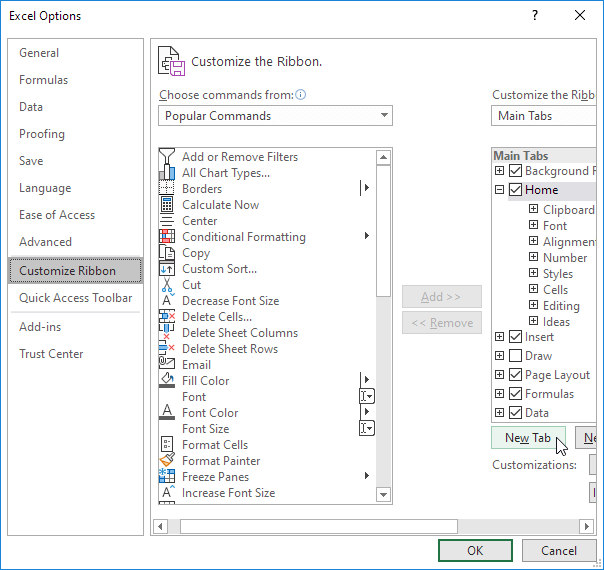
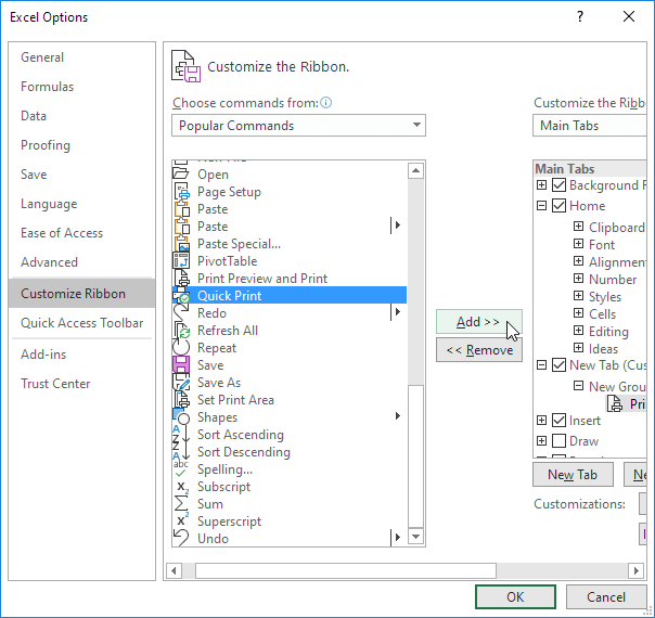
3. Add the commands you like.
4. Rename the tab and group.
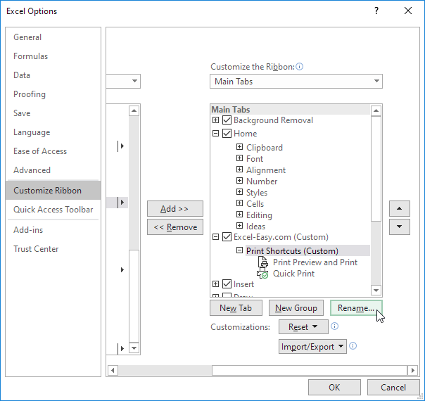
Note: you can also add new groups to existing tabs. To hide a tab, uncheck the corresponding check box. Click Reset, Reset all customizations, to delete all Ribbon customizations.
5. Click OK.
Result.
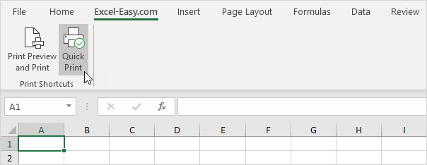
The ribbon in Excel can be customized. You can easily create your own tab and add commands to it.
1. Right click anywhere on the ribbon, and then click Customize the Ribbon.

2. Click New Tab.

3. Add the commands you like.

4. Rename the tab and group.

Note: you can also add new groups to existing tabs. To hide a tab, uncheck the corresponding check box. Click Reset, Reset all customizations, to delete all Ribbon customizations.
5. Click OK.
Result.

Developer Tab
Turn on the Developer tab in Excel if you want to create a macro, export and import XML files or insert controls.
To turn on the Developer tab, execute the following steps.
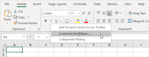
1. Right click anywhere on the ribbon, and then click Customize the Ribbon.
2. Under Customize the Ribbon, on the right side of the dialog box, select Main tabs (if necessary).
3. Check the Developer check box.
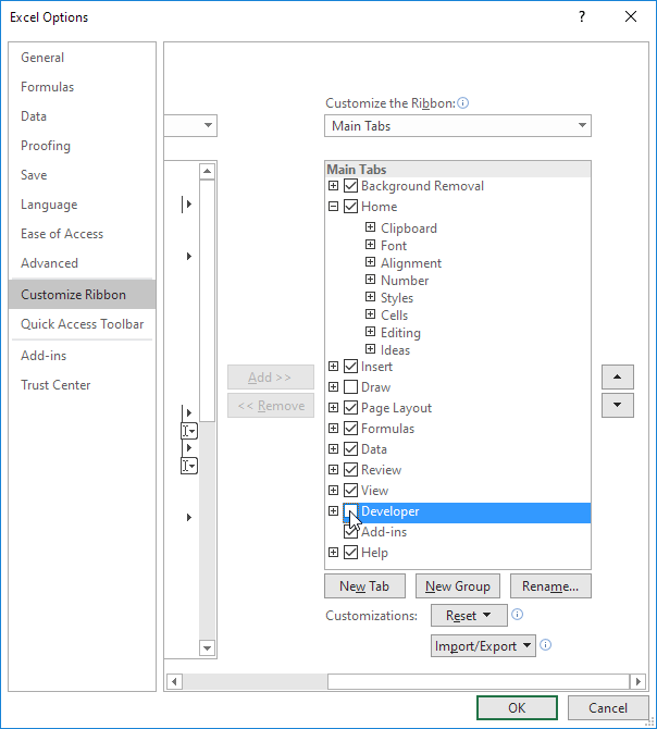
4. Click OK.
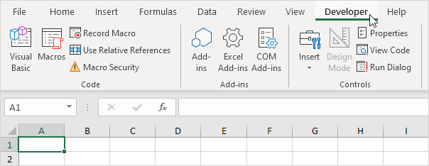
5. You can find the Developer tab next to the View tab.
Turn on the Developer tab in Excel if you want to create a macro, export and import XML files or insert controls.
To turn on the Developer tab, execute the following steps.
1. Right click anywhere on the ribbon, and then click Customize the Ribbon.

2. Under Customize the Ribbon, on the right side of the dialog box, select Main tabs (if necessary).
3. Check the Developer check box.

4. Click OK.
5. You can find the Developer tab next to the View tab.

Status Bar
1:- Status Bar 101
2:- Customize Status Bar
3:- Status Bar Secrets
The status bar in Excel can be quite useful. By default, the status bar at the bottom of the window displays the average, count and sum of selected cells.
1:- Status Bar 101
2:- Customize Status Bar
3:- Status Bar Secrets
The status bar in Excel can be quite useful. By default, the status bar at the bottom of the window displays the average, count and sum of selected cells.
Status Bar 101
The status bar in Excel can do the math for you.
1. Select the range A1:A3.

2. Look at the status bar to see the average, count and sum of these cells.

3. To quickly change the workbook view, use the 3 view shortcuts on the status bar.

Note: visit our page about workbook views to learn more about this topic.
4. Use the zoom slider on the status bar to quickly zoom in or out to a preset percentage.

Note: use the ribbon to zoom to a specific percentage or to zoom to a selection.
The status bar in Excel can do the math for you.
1. Select the range A1:A3.

2. Look at the status bar to see the average, count and sum of these cells.

3. To quickly change the workbook view, use the 3 view shortcuts on the status bar.

Note: visit our page about workbook views to learn more about this topic.
4. Use the zoom slider on the status bar to quickly zoom in or out to a preset percentage.

Note: use the ribbon to zoom to a specific percentage or to zoom to a selection.
Customize Status Bar
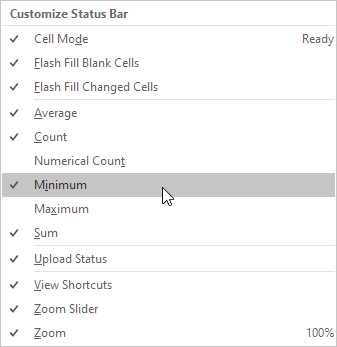
Many status bar options are selected by default. Right click the status bar to activate even more options.
1. Right click the status bar.
2. For example, click Caps Lock.
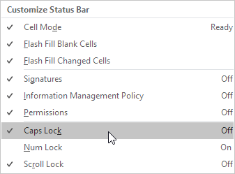
Note: this doesn't turn on Caps Lock (see image above, Caps Lock is still turned off). The status bar displays the Caps Lock status now.
3. Press the Caps Lock key on your keyboard.
4. Excel displays the text Caps Lock in the status bar.

5. Right click the status bar.
6. For example, click Minimum.
7. Select the range A1:A3.

8. Look at the status bar to see the average, count, minimum and sum of these cells.

Many status bar options are selected by default. Right click the status bar to activate even more options.
1. Right click the status bar.
2. For example, click Caps Lock.

Note: this doesn't turn on Caps Lock (see image above, Caps Lock is still turned off). The status bar displays the Caps Lock status now.
3. Press the Caps Lock key on your keyboard.
4. Excel displays the text Caps Lock in the status bar.

5. Right click the status bar.
6. For example, click Minimum.

7. Select the range A1:A3.

8. Look at the status bar to see the average, count, minimum and sum of these cells.

Status Bar Secrets
Here's a little secret: Excel uses the status bar in many other situations. If you don't like this, hide the status bar.
1. For example, filter a table.
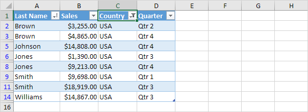
2. Excel uses the status bar to display the number of visible records.

3. Hover over a cell with one or more comments.
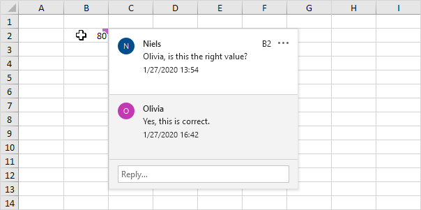
4. Excel uses the status bar to display the name of the author.

5. If you have Excel 2016, use the shortcut CTRL + SHIFT + F1 to hide the ribbon and the status bar.
6. To only hide the status bar, add the following code line to the Workbook Open Event:
Application.DisplayStatusBar = False7. Use the StatusBar property in Excel VBA to display a message on the status bar.
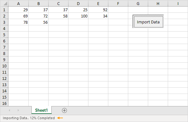
Note: if you're new to Excel, you can skip step 6 and step 7.
Here's a little secret: Excel uses the status bar in many other situations. If you don't like this, hide the status bar.
1. For example, filter a table.

2. Excel uses the status bar to display the number of visible records.

3. Hover over a cell with one or more comments.

4. Excel uses the status bar to display the name of the author.

5. If you have Excel 2016, use the shortcut CTRL + SHIFT + F1 to hide the ribbon and the status bar.
6. To only hide the status bar, add the following code line to the Workbook Open Event:
7. Use the StatusBar property in Excel VBA to display a message on the status bar.

Note: if you're new to Excel, you can skip step 6 and step 7.
Checkbox
1:- Insert a Checkbox
2:- Link a Checkbox
3:- Create a Checklist
4:- Dynamic Chart
5:- Delete Checkboxes
6:- Powerful Checkboxes
Inserting a checkbox in Excel is easy. For example, use checkboxes to create a checklist or a dynamic chart. You can also insert a check mark symbol.
1:- Insert a Checkbox
2:- Link a Checkbox
3:- Create a Checklist
4:- Dynamic Chart
5:- Delete Checkboxes
6:- Powerful Checkboxes
Inserting a checkbox in Excel is easy. For example, use checkboxes to create a checklist or a dynamic chart. You can also insert a check mark symbol.
Insert a Checkbox
To insert a checkbox, execute the following steps.
1. On the Developer tab, in the Controls group, click Insert.

2. Click Check Box in the Form Controls section.

3. For example, draw a checkbox in cell B2.

4. To remove "Check Box 1", right click the checkbox, click the text and delete it.

To insert a checkbox, execute the following steps.
1. On the Developer tab, in the Controls group, click Insert.

2. Click Check Box in the Form Controls section.

3. For example, draw a checkbox in cell B2.

4. To remove "Check Box 1", right click the checkbox, click the text and delete it.

Link a Checkbox
To link a checkbox to a cell, execute the following steps.
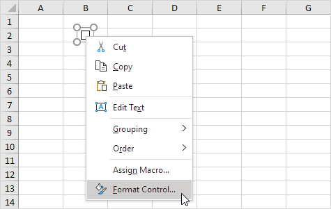
1. Right click the checkbox and click Format Control.
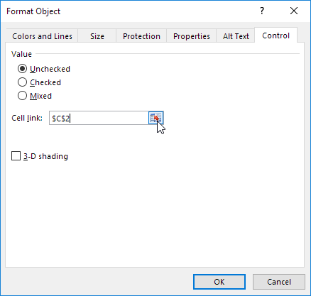
2. Link the checkbox to cell C2.
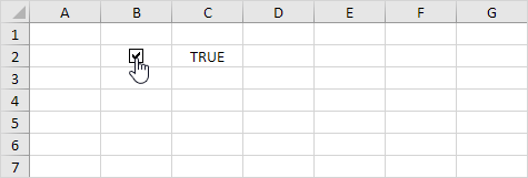
3. Test the checkbox.
4. Hide column C.
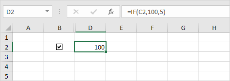
5. For example, enter a simple IF function.
6. Uncheck the checkbox.
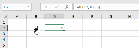
Note: read on for some cool examples.
Create a Checklist
To link a checkbox to a cell, execute the following steps.
1. Right click the checkbox and click Format Control.

2. Link the checkbox to cell C2.

3. Test the checkbox.

4. Hide column C.
5. For example, enter a simple IF function.

6. Uncheck the checkbox.

Note: read on for some cool examples.
Create a Checklist
To create a checklist, execute the following steps.
1. Draw a checkbox in cell B2.
2. Click on the lower right corner of cell B2 and drag it down to cell B11.
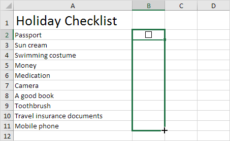
3. Right click the first checkbox and click Format Control.
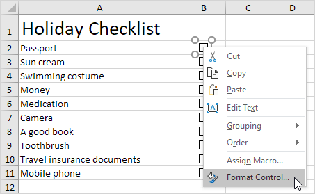
4. Link the checkbox to the cell next to it (cell C2).
5. Repeat step 4 for the other checkboxes.
6. Insert a COUNTIF function to count the number of items packed.
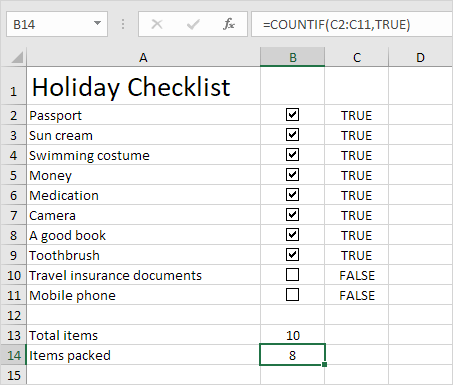
7. Hide column C.
8. Insert an IF function that determines if you're good to go.
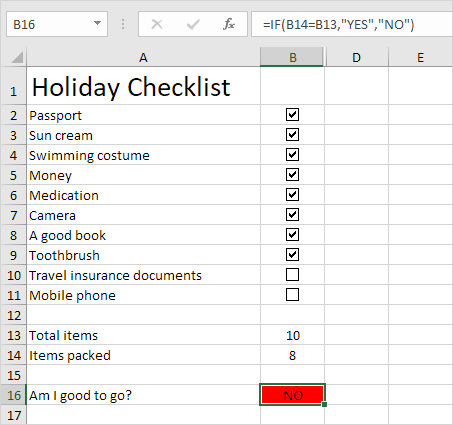
9. Click all the checkboxes.
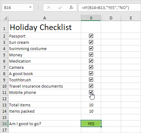
Note: we created a conditional formatting rule to automatically change the background color of cell B16. Try it yourself. Download the Excel file and test the checklist (second sheet).
To create a checklist, execute the following steps.
1. Draw a checkbox in cell B2.
2. Click on the lower right corner of cell B2 and drag it down to cell B11.

3. Right click the first checkbox and click Format Control.

4. Link the checkbox to the cell next to it (cell C2).
5. Repeat step 4 for the other checkboxes.
6. Insert a COUNTIF function to count the number of items packed.

7. Hide column C.
8. Insert an IF function that determines if you're good to go.

9. Click all the checkboxes.

Note: we created a conditional formatting rule to automatically change the background color of cell B16. Try it yourself. Download the Excel file and test the checklist (second sheet).
Dynamic Chart
Let's take a look at one more cool example that uses checkboxes. A dynamic chart.
1. For example, create a combination chart with two data series (Rainy Days and Profit).
2. Add two checkboxes.
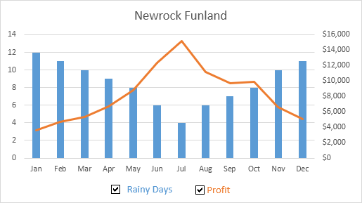
3. Right click the first checkbox and click Format Control. Link this checkbox to cell B15.
4. Right click the second checkbox and click Format Control. Link this checkbox to cell C15.
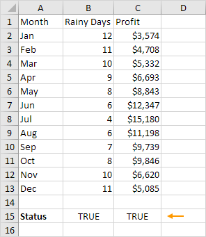
5. Uncheck the second checkbox. Cell C15 below changes to FALSE.
We're now going to create two new data series.
6. Insert the IF function shown below. Use the fill handle to copy this formula down to cell F13.
7. Repeat this step for the new Profit data series.
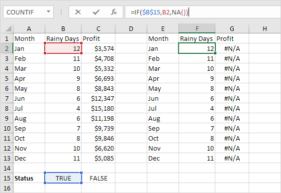
Explanation: if the checkbox is checked, the old and new data series are the same. If the checkbox is unchecked, the new data series changes to a range with #N/A errors.
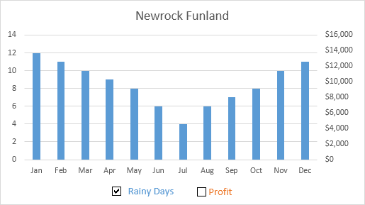
8. Use the new data series to create the combination chart. To achieve this, select the chart, right click, and then click Select Data.
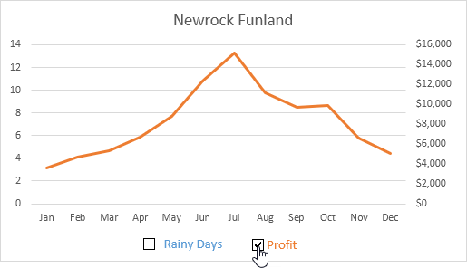
9. Uncheck the first checkbox and check the second checkbox.
Note: try it yourself. Download the Excel file and test the dynamic chart (third sheet).
Delete Checkboxes
Let's take a look at one more cool example that uses checkboxes. A dynamic chart.
1. For example, create a combination chart with two data series (Rainy Days and Profit).
2. Add two checkboxes.

3. Right click the first checkbox and click Format Control. Link this checkbox to cell B15.
4. Right click the second checkbox and click Format Control. Link this checkbox to cell C15.

5. Uncheck the second checkbox. Cell C15 below changes to FALSE.
We're now going to create two new data series.
6. Insert the IF function shown below. Use the fill handle to copy this formula down to cell F13.
7. Repeat this step for the new Profit data series.

Explanation: if the checkbox is checked, the old and new data series are the same. If the checkbox is unchecked, the new data series changes to a range with #N/A errors.
8. Use the new data series to create the combination chart. To achieve this, select the chart, right click, and then click Select Data.

9. Uncheck the first checkbox and check the second checkbox.

Note: try it yourself. Download the Excel file and test the dynamic chart (third sheet).
Delete Checkboxes
To delete multiple checkboxes, execute the following steps.
1. Hold down CTRL and use the left mouse button to select multiple checkboxes.
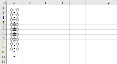
2. Press Delete.
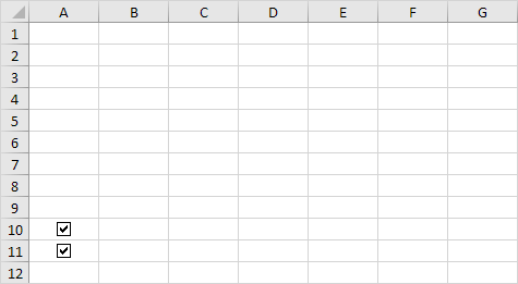
To delete multiple checkboxes, execute the following steps.
1. Hold down CTRL and use the left mouse button to select multiple checkboxes.

2. Press Delete.

Powerful Checkboxes
Finally, you can use VBA to create powerful checkboxes in Excel. Instead of inserting a Form control, simply insert an ActiveX control.
1. Insert a checkbox (ActiveX control).
2. At step 6, you can add your own code lines to automate all kinds of tasks. For example, add the following code lines to hide and unhide column F.
If CheckBox1.Value = True Then Columns("F").Hidden = True
If CheckBox1.Value = False Then Columns("F").Hidden = False


Note: maybe coding is one step too far for you at this stage, but it shows you one of the many other powerful features Excel has to offer.
Finally, you can use VBA to create powerful checkboxes in Excel. Instead of inserting a Form control, simply insert an ActiveX control.
1. Insert a checkbox (ActiveX control).
2. At step 6, you can add your own code lines to automate all kinds of tasks. For example, add the following code lines to hide and unhide column F.
If CheckBox1.Value = False Then Columns("F").Hidden = False


Note: maybe coding is one step too far for you at this stage, but it shows you one of the many other powerful features Excel has to offer.


0 মন্তব্যসমূহ